
The steps to follow to use machine learning models are:
- Import libraries you need to work with in your project
- Load your dataset
- Split the dataset to train, and test sets. The goal is to train your model on the training sets, and compute the accuracy of the model on the test sets, which was not discovered yet by the model (to be the most realistic)
- Normalize your data train, and then infer this transformation to the test sets
- Fit the model
- Predict
- Evaluate the model
In “fit” and “predict” steps, you can use several models, and evaluate them, to keep the most performing one.
Python libraries:
import pandas as pd
import numpy as np
from sklearn.preprocessing import StandardScaler
from sklearn.preprocessing import normalize, Normalizer
from sklearn.linear_model import LinearRegression, Lasso
from sklearn.metrics import r2_score, explained_variance_score, mean_squared_error, mean_absolute_error
from sklearn.metrics import mean_absolute_percentage_error, median_absolute_error
import matplotlib.pyplot as plt
import seaborn as sns
Here, we train a model to guess a comfortable boot size for a dog, based on the size of the harness that fits them:
import pandas

# Let's make a dictionary of data for boot sizes
# and harness sizes in cm
data = {
    'boot_size' : [ 39, 38, 37, 39, 38, 35, 37, 36, 35, 40,
                    40, 36, 38, 39, 42, 42, 36, 36, 35, 41,
                    42, 38, 37, 35, 40, 36, 35, 39, 41, 37,
                    35, 41, 39, 41, 42, 42, 36, 37, 37, 39,
                    42, 35, 36, 41, 41, 41, 39, 39, 35, 39
 ],
    'harness_size': [ 58, 58, 52, 58, 57, 52, 55, 53, 49, 54,
                59, 56, 53, 58, 57, 58, 56, 51, 50, 59,
                59, 59, 55, 50, 55, 52, 53, 54, 61, 56,
                55, 60, 57, 56, 61, 58, 53, 57, 57, 55,
                60, 51, 52, 56, 55, 57, 58, 57, 51, 59
                ]
}

# Convert it into a table using pandas
dataset = pandas.DataFrame(data)

# Print the data
dataset.head()
boot_size	harness_size
0	39	58
1	38	58
2	37	52
3	39	58
4	38	57
Let’s take a very simple model called OLS. This is just a straight line (sometimes called a trendline).
# Load a library to do the hard work for us
import statsmodels.formula.api as smf

# First, we define our formula using a special syntax
# This says that boot_size is explained by harness_size
formula = "boot_size ~ harness_size"

# Create the model, but don't train it yet
model = smf.ols(formula = formula, data = dataset)
OLS models have two parameters (a slope and an offset), but these haven’t been set in our model yet. We need to train (fit) our model to find these values so that the model can reliably estimate dogs’ boot size based on their harness size.
The following code fits our model to data you’ve now seen:
# Train (fit) the model so that it creates a line that
# fits our data. This method does the hard work for us.
fitted_model = model.fit()

# Print information about our model now it has been fit
print("The following model parameters have been found:\n" +
        f"Line slope: {fitted_model.params[1]}\n"+
        f"Line Intercept: {fitted_model.params[0]}")
The following model parameters have been found:
Line slope: 0.585925416738271
Line Intercept: 5.71910981268259
Notice how training the model set its parameters. We could interpret these directly, but it’s simpler to see it as a graph:
import matplotlib.pyplot as plt

# Show a scatter plot of the data points and add the fitted line
plt.scatter(dataset["harness_size"], dataset["boot_size"])
plt.plot(dataset["harness_size"], fitted_model.params[1] * dataset["harness_size"] + fitted_model.params[0], 'r', label='Fitted line')

# add labels and legend
plt.xlabel("harness_size")
plt.ylabel("boot_size")
plt.legend()
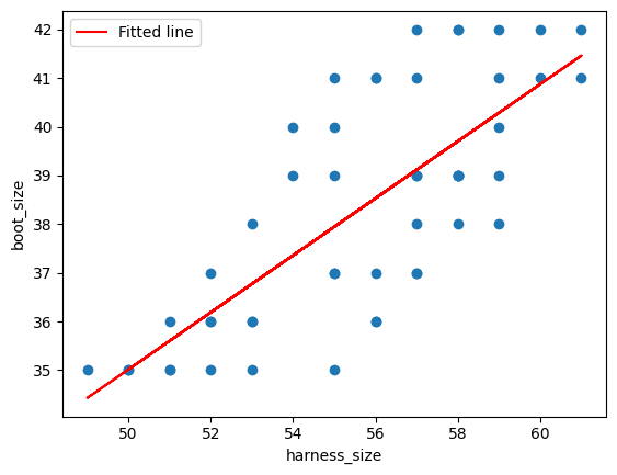
The graph above shows our original data as circles with a red line through it. The red line shows our model.
Now that we’ve finished training, we can use our model to predict a dog’s boot size from their harness size.
# harness_size states the size of the harness we are interested in
harness_size = { 'harness_size' : [52.5] }

# Use the model to predict what size of boots the dog will fit
approximate_boot_size = fitted_model.predict(harness_size)

# Print the result
print("Estimated approximate_boot_size:")
print(approximate_boot_size[0])
Estimated approximate_boot_size:
36.48019419144182