
Principal Component Analysis (PCA) is a widely used linear dimensionality reduction technique (of type Feature Extraction) used for reducing the dimensionality of datasets containing many correlated variables while preserving most of the variability in the data.
Here’s how PCA works:
- Data Standardization (Scaling): PCA is sensitive to the scale of the variables, so it’s common practice to standardize the data by centering each variable around its mean and scaling it to have unit variance.
- Compute Covariance Matrix: PCA analyzes the variance-covariance matrix (or the correlation matrix) of the standardized data. This matrix shows how each variable in the dataset varies with respect to every other variable.
- Eigenvalue Decomposition or Singular Value Decomposition (SVD): PCA then calculates the eigenvectors and eigenvalues of the covariance matrix. The eigenvectors represent the directions (or principal components) of maximum variance in the data, while the eigenvalues represent the magnitude of variance along these directions.
- Select Principal Components: PCA sorts the eigenvectors based on their corresponding eigenvalues in descending order. The principal components are then selected from these sorted eigenvectors. Typically, one retains only the top k eigenvectors (principal components) that capture the most variance in the data.
- Transform Data: Finally, PCA transforms the original data into the new lower-dimensional space spanned by the selected principal components. This transformation is achieved by projecting the data onto the principal components.
Each of the “new” variables after PCA are all independent of one another.
PCA has several applications:
- Dimensionality Reduction: PCA is primarily used for reducing the dimensionality of high-dimensional datasets, making it easier to visualize and analyze data while retaining most of the variability.
- Data Visualization: PCA can be used to visualize high-dimensional data in lower-dimensional space (e.g., 2D or 3D) while preserving the structure and relationships between data points.
- Noise Reduction: PCA can help in removing noise and redundancy from the data by focusing on the principal components that capture the most significant variability.
- Feature Engineering: PCA can also be used as a feature engineering technique to create new features that capture the most important information in the original dataset.
However, it’s essential to note that PCA is a linear technique and may not capture complex nonlinear relationships in the data. Additionally, interpretability of the principal components might be challenging, especially when dealing with a large number of features.
Python Library:
from sklearn.decomposition import PCA
Example:
import numpy as np
from scipy.stats import zscore
from sklearn.decomposition import PCA
import matplotlib.pyplot as plt
%matplotlib inline
import seaborn as sns
X = data.drop('mpg', axis=1)
y = data['mpg']
X_scaled = X.apply(zscore)
covMatrix = np.cov(X_scaled, rowvar=False)
print(covMatrix)
#
pca = PCA(n_components=6)
pca.fit(X_scaled)
# the eigen Values
print(pca.explained_variance_)
# the eigen Vectors
print(pca.components_)
# the percentage of variation explained by each eigen Vector
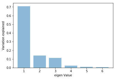
print(pca.explained_variance_ratio_)
plt.bar(list(range(1,7)),pca.explained_variance_ratio_,alpha=0.5, align='center')
plt.ylabel('Variation explained')
plt.xlabel('eigen Value')
plt.show()
plt.step(list(range(1,7)),np.cumsum(pca.explained_variance_ratio_), where='mid')
plt.ylabel('Cum of variation explained')
plt.xlabel('eigen Value')
plt.show()
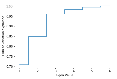
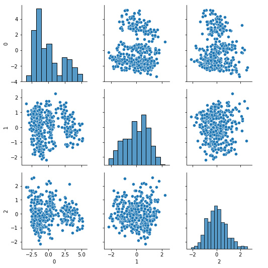
Three dimensions seems very reasonable. With 3 variables we can explain over 95% of the variation in the original data!
pca3 = PCA(n_components=3)
pca3.fit(XScaled)
print(pca3.components_)
print(pca3.explained_variance_ratio_)
Xpca3 = pca3.transform(XScaled)
[[ 0.45509041  0.46913807  0.46318283  0.44618821 -0.32466834 -0.23188446]
 [ 0.18276349  0.16077095  0.0139189   0.25676595  0.21039209  0.9112425 ]
 [ 0.17104591  0.13443134 -0.12440857  0.27156481  0.86752316 -0.33294164]]
[0.70884563 0.13976166 0.11221664]
sns.pairplot(pd.DataFrame(Xpca3))
regression_model_pca = LinearRegression()
regression_model_pca.fit(Xpca3, y)
regression_model_pca.score(Xpca3, y)
0.7799909620572006
An out of sample (on test data), with the 3 independent variables is likely to do better since that would be less of an over-fit.