
Gradient Descent is an optimization algorithm commonly used in machine learning and deep learning to minimize the loss function and find the optimal parameters (weights and biases) of a model. It’s based on the principle of iteratively moving in the direction of the steepest descent of the loss function with respect to the model parameters.
Here’s how Gradient Descent works:
- Initialization: It starts with an initial set of parameters (weights and biases) for the model.
- Compute Gradient: It computes the gradient of the loss function with respect to each parameter. The gradient represents the direction of the steepest increase of the loss function, so the negative gradient points in the direction of the steepest decrease.
- Update Parameters: It updates the parameters in the opposite direction of the gradient to minimize the loss function. The magnitude of the update is determined by the learning rate, which controls the size of the steps taken during optimization.
- Repeat: Steps 2 and 3 are repeated iteratively until convergence or until a predefined number of iterations is reached.
There are different variants of Gradient Descent, such as:
- Batch Gradient Descent: Computes the gradient using the entire dataset.
- Stochastic Gradient Descent (SGD): Computes the gradient using only one sample from the dataset at a time. It’s faster but more noisy compared to batch gradient descent.
- Mini-batch Gradient Descent: Computes the gradient using a small random subset (mini-batch) of the dataset. It combines the advantages of batch and stochastic gradient descent.
Let’s go through a step-by-step example to understand how it works, using a simple function.
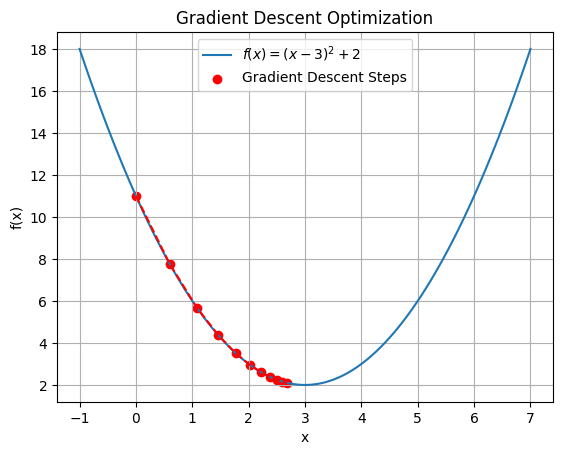
Example: Minimizing a Quadratic Function
Consider the quadratic function:
\( f(x) = (x – 3)^2 + 2 \)
Objective: Find the value of ( x ) that minimizes ( f(x) ).
Step 1: Initialization
Start with an initial guess for ( x ). Let’s say ( x_0 = 0 ).
Step 2: Compute the Gradient
The gradient of the function ( f(x) ) with respect to ( x ) is the derivative of the function. For our function:
\( f(x) = (x – 3)^2 + 2 \)The derivative (gradient) is:
\( f'(x) = \frac{d}{dx}[(x – 3)^2 + 2] = 2(x – 3) \)Step 3: Update Rule
Use the gradient to update the current value of ( x ). The update rule is:
\( x_{new} = x_{old} – \alpha f'(x_{old}) \)where \( ( \alpha )\) is the learning rate, a small positive number that controls the step size. Let’s set \( ( \alpha = 0.1 )\) .
Step 4: Iteration
Repeat the process until convergence (when the change in ( x ) is very small).
Iteration 1:
- Initial ( x ): ( x_0 = 0 )
- Compute gradient: \( ( f'(x_0) = 2(0 – 3) = -6 ) \)
- Update ( x ): \( ( x_1 = x_0 – \alpha f'(x_0) = 0 – 0.1(-6) = 0.6 ) \)
Iteration 2:
- New ( x ): ( x_1 = 0.6 )
- Compute gradient: \( ( f'(x_1) = 2(0.6 – 3) = -4.8 ) \)
- Update ( x ): \( ( x_2 = x_1 – \alpha f'(x_1) = 0.6 – 0.1(-4.8) = 1.08 ) \)
Iteration 3:
- New ( x ): ( x_2 = 1.08 )
- Compute gradient: \( ( f'(x_2) = 2(1.08 – 3) = -3.84 ) \)
- Update ( x ): \( ( x_3 = x_2 – \alpha f'(x_2) = 1.08 – 0.1(-3.84) = 1.464 ) \)
And so on…
Step 5: Convergence
Continue the iterations until the change in ( x ) is negligible. At convergence, ( x ) will be close to the value that minimizes the function ( f(x) ).
For our example, as we keep iterating, ( x ) will approach 3, which is the minimum point of ( f(x) ).
Key Points to Remember
- Gradient: Indicates the direction of the steepest ascent. We move in the opposite direction to minimize the function.
- Learning Rate ( \( \alpha \) ): Controls the step size. If it’s too large, the algorithm may overshoot the minimum; if too small, the convergence will be slow.
- Convergence: The process is repeated until the function’s value or the changes in ( x ) become very small.
import numpy as np
import matplotlib.pyplot as plt

# Define the function and its derivative
def f(x):
    return (x - 3)**2 + 2

def f_prime(x):
    return 2 * (x - 3)

# Gradient descent parameters
x_init = 0.0  # Initial guess
alpha = 0.1   # Learning rate
iterations = 10  # Number of iterations

# Storage for plotting
x_values = [x_init]
f_values = [f(x_init)]

# Gradient Descent
x = x_init
for _ in range(iterations):
    x -= alpha * f_prime(x)
    x_values.append(x)
    f_values.append(f(x))

# Plotting
x_plot = np.linspace(-1, 7, 100)
y_plot = f(x_plot)

plt.plot(x_plot, y_plot, label='$f(x) = (x - 3)^2 + 2$')
plt.scatter(x_values, f_values, color='red', label='Gradient Descent Steps')
plt.plot(x_values, f_values, color='red', linestyle='dashed')
plt.xlabel('x')
plt.ylabel('f(x)')
plt.title('Gradient Descent Optimization')
plt.legend()
plt.grid(True)
plt.show()
In addition to Stochastic Gradient Descent (SGD), several other optimization algorithms can be used for minimizing the loss function in model training. These algorithms often include improvements or modifications to the basic gradient descent to improve convergence speed, stability, or accuracy. Here are some popular alternatives:
1. Batch Gradient Descent
- Description: Uses the entire dataset to compute the gradient of the cost function and update the parameters.
- Pros: Converges smoothly.
- Cons: Can be very slow and computationally expensive, especially with large datasets.
2. Mini-Batch Gradient Descent
- Description: Splits the dataset into smaller batches and performs an update for each batch.
- Pros: Provides a balance between the stability of batch gradient descent and the efficiency of SGD.
- Cons: Choosing the appropriate batch size can be challenging.
3. Momentum
- Description: Accelerates SGD by moving in the direction of the accumulated gradient of past steps. It adds a fraction of the previous update to the current update.
- Pros: Helps accelerate gradients vectors and reduces oscillation.
- Cons: Requires an additional parameter to tune (momentum term).
4. Nesterov Accelerated Gradient (NAG)
- Description: A variant of momentum where the gradient is computed after the current velocity is applied.
- Pros: Provides more accurate updates and typically converges faster than standard momentum.
- Cons: Adds complexity and requires careful tuning.
5. Adagrad (Adaptive Gradient Algorithm)
- Description: Adapts the learning rate to the parameters, performing larger updates for infrequent parameters and smaller updates for frequent ones.
- Pros: Handles sparse data well and requires less tuning of the learning rate.
- Cons: Accumulated gradients can lead to a very small learning rate over time, slowing down the convergence.
6. RMSprop (Root Mean Square Propagation)
- Description: Adapts the learning rate for each parameter using a moving average of squared gradients.
- Pros: Prevents the learning rate from becoming too small and works well for online and non-stationary problems.
- Cons: Requires tuning of the decay parameter.
7. Adam (Adaptive Moment Estimation)
- Description: Combines the benefits of Adagrad and RMSprop. It computes adaptive learning rates for each parameter and maintains moving averages of both the gradients and their squares.
- Pros: Often works well out-of-the-box and is widely used in practice.
- Cons: Requires tuning of additional hyperparameters (like beta1, beta2).
8. Adadelta
- Description: An extension of Adagrad that seeks to reduce its aggressive, monotonically decreasing learning rate.
- Pros: It has an adaptive learning rate that doesn’t decay over time as in Adagrad.
- Cons: Can be sensitive to hyperparameters.
9. AdaMax
- Description: A variant of Adam based on the infinity norm.
- Pros: Can handle very large gradients better.
- Cons: Similar limitations as Adam but may work better in some specific cases.
10. Nadam
- Description: Combines Adam and Nesterov momentum.
- Pros: Can converge faster and smoother than Adam.
- Cons: More complex and requires tuning additional hyperparameters.
11. LBFGS (Limited-memory Broyden–Fletcher–Goldfarb–Shanno)
- Description: An optimization algorithm in the family of quasi-Newton methods. It approximates the BFGS algorithm using limited computer memory.
- Pros: Can be very effective for smaller datasets or with a strong second-order approximation.
- Cons: Computationally expensive and less suitable for large datasets or deep networks.
Choosing the Right Optimizer
The choice of optimizer can depend on various factors, such as the size of the dataset, the architecture of the neural network, and the specific problem being solved. In practice, Adam is often a good starting point because it generally performs well across a wide range of problems. However, for specific cases, experimenting with different optimizers and tuning their hyperparameters may lead to better results.
Let’s walk through an example of training a simple linear regression model using Stochastic Gradient Descent (SGD) in Python. We’ll use a synthetic dataset for this example.
Problem Setup
We’ll create a dataset where the target variable ( y ) is a linear function of the input feature ( x ) with some added noise. The model will attempt to learn the relationship between ( x ) and ( y ).
Model
The model we’re training is a simple linear regression model, represented as:
\( y = w \cdot x + b \)Where:
- \( w \) is the weight (slope)
- \( b \) is the bias (intercept)
SGD Optimization
We’ll use SGD to minimize the Mean Squared Error (MSE) loss function, which measures the average squared difference between the predicted and actual values.
Step-by-Step Implementation
import numpy as np
import matplotlib.pyplot as plt

# Generate synthetic data
np.random.seed(42)
X = 2 * np.random.rand(100, 1)
y = 4 + 3 * X + np.random.randn(100, 1)

# Hyperparameters
learning_rate = 0.01
n_iterations = 1000
m = len(X)  # Number of samples

# Initialize parameters (weights and bias)
w = np.random.randn(1)
b = np.zeros(1)

# SGD Optimization
for iteration in range(n_iterations):
    # Shuffle the data
    shuffled_indices = np.random.permutation(m)
    X_shuffled = X[shuffled_indices]
    y_shuffled = y[shuffled_indices]

    for i in range(m):
        xi = X_shuffled[i:i+1]
        yi = y_shuffled[i:i+1]

        # Compute gradients
        y_pred = xi * w + b
        error = y_pred - yi

        grad_w = 2 * xi.T.dot(error)
        grad_b = 2 * error

        # Update parameters
        w -= learning_rate * grad_w
        b -= learning_rate * grad_b

print(f"Trained weights: {w}")
print(f"Trained bias: {b}")

# Plotting the results
plt.scatter(X, y, color='blue', label='Data points')
plt.plot(X, X * w + b, color='red', label='Fitted line')
plt.xlabel('x')
plt.ylabel('y')
plt.title('Linear Regression using SGD')
plt.legend()
plt.grid(True)
plt.show()
Explanation
- Synthetic Data Generation:
- We generate 100 random points for ( x ) and compute the corresponding ( y ) values using a linear function with some noise.
- Hyperparameters:
learning_rate: Determines the step size in the gradient descent update.n_iterations: The number of iterations to run SGD.m: The number of samples in the dataset.
- Parameter Initialization:
- We initialize the weight ( w ) and bias ( b ) randomly.
- SGD Optimization Loop:
- Data Shuffling: Before each epoch, the data is shuffled to ensure that the model doesn’t see the same data order each time.
- Mini-Batch Gradient Descent: For each sample in the shuffled dataset, we compute the predicted value, calculate the gradient of the loss function with respect to the parameters, and update the parameters accordingly.
- Parameter Update:
- The parameters ( w ) and ( b ) are updated using the gradients and the learning rate.
- Plotting the Results:
- After training, we plot the original data points and the fitted line representing the learned linear relationship.
Output
The output will display the learned weights and bias, and the plot will show the best-fit line through the data points.
This simple example demonstrates how SGD can be used to train a linear regression model. The approach can be extended to more complex models and datasets by adjusting the model, loss function, and optimization process accordingly.