t-SNE, which stands for t-distributed Stochastic Neighbor Embedding, is a popular dimensionality reduction technique (of type Feature Extraction) used in machine learning and data visualization. It is particularly useful for visualizing high-dimensional data in a lower-dimensional space, typically two or three dimensions, while preserving the local structure of the data as much as possible.
The main idea behind t-SNE is to map high-dimensional data points to a lower-dimensional space in such a way that similar points in the high-dimensional space are represented as nearby points in the low-dimensional space, while dissimilar points are represented as distant points. This is achieved by modeling the similarity between data points in both the high-dimensional and low-dimensional spaces using probability distributions and minimizing the mismatch between them.
t-SNE is commonly used in exploratory data analysis, clustering, and visualization tasks, especially when dealing with complex and nonlinear relationships in the data. However, it’s important to note that t-SNE is computationally expensive and may not always preserve global structures accurately, especially in cases of very high-dimensional data. Additionally, t-SNE is sensitive to its hyperparameters, and different parameter settings can lead to different visualizations.
Example
import pandas as pd
import numpy as np
import matplotlib.pyplot as plt
%matplotlib inline
import seaborn as sns

sns.set_theme()

pd.set_option('display.max_rows', 200)
pd.set_option('display.max_columns', None)
pd.set_option('display.float_format', '{:,.2f}'.format)

from scipy.stats import zscore
from sklearn.manifold import TSNE

# X is the numeric columns
X_scaled = X.apply(zscore)

tsne = TSNE(n_components=2, random_state=1)
X_reduced = tsne.fit_transform(X_scaled)

df = pd.DataFrame(X_reduced, columns=['component1', 'component2'])

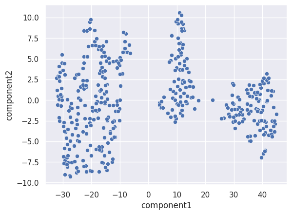
sns.scatterplot(x=df['component1'], y=df['component2'])

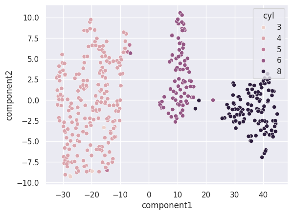
sns.scatterplot(x=df['component1'], y=df['component2'], hue=data['cyl'])


