The key characteristics of a binomial distribution are:
- Two Outcomes: Each trial has only two possible outcomes, typically labeled as “success” and “failure.”
- Fixed Number of Trials: The number of trials (experiments) is fixed in advance.
- Independent Trials: Each trial is independent of the others, meaning the outcome of one trial does not influence the outcomes of the others.
- Constant Probability: The probability of success is the same for each trial.
The probability mass function (PMF) of the binomial distribution is given by the formula:

where:
The mean (μ) and variance of a binomial distribution are given by:
\( \mu = n \cdot p\) \( \sigma^2 = n \cdot p \cdot (1 – p)
\)
Binomial distributions are commonly used in statistics and probability theory to model scenarios involving repeated, independent trials with binary outcomes. Examples include coin flips, success/failure experiments, and certain types of counting processes.
In real life, the concept is used for:
- Finding the quantity of raw and used materials while making a product.
- Taking a survey of positive and negative reviews from the public for any specific product or place.
- By using the YES/ NO survey, we can check whether the number of persons views the particular channel.
- To find the number of male and female employees in an organisation.
- The number of votes collected by a candidate in an election is counted based on 0 or 1 probability.
Binomial Distribution Vs Normal Distribution
The main difference between the binomial distribution and the normal distribution is that binomial distribution is discrete, whereas the normal distribution is continuous. It means that the binomial distribution has a finite number of events, whereas the normal distribution has an infinite number of events. In case, if the sample size for the binomial distribution is very large, then the distribution curve for the binomial distribution is similar to the normal distribution curve.
binomial distribution in Python
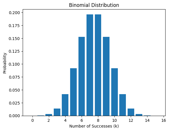
If you want to draw a binomial distribution in Python, you can use the scipy.stats module along with matplotlib for visualization. Here’s an example:
import numpy as np
import matplotlib.pyplot as plt
from scipy.stats import binom

# Set the parameters for the binomial distribution
n = 15  # Number of trials
p = 0.5  # Probability of success

# Generate x values (number of successes)
x = np.arange(0, n+1)

# Calculate the probability mass function (PMF) for each x
pmf = binom.pmf(x, n, p)

# Plot the binomial distribution
plt.bar(x, pmf)
plt.xlabel('Number of Successes (k)')
plt.ylabel('Probability')
plt.title('Binomial Distribution')
plt.show()


