SequentialFeatureSelector is a feature selection technique. It is part of the feature_selection module and is used for selecting a subset of features from the original feature set. This technique follows a forward or backward sequential selection strategy.
Here’s a brief overview:
- Forward Sequential Selection: It starts with an empty set of features and iteratively adds features to the set based on their contribution to the model’s performance.
- Backward Sequential Selection: It starts with the full set of features and iteratively removes features from the set based on their contribution to the model’s performance.
SequentialFeatureSelector is often used in conjunction with machine learning models to identify the most relevant features for a given task. It evaluates different combinations of features by fitting the model on subsets of features and selecting the set that results in the best performance according to a specified criterion (e.g., accuracy, precision, recall).
Here’s a basic example of how to use SequentialFeatureSelector with mlxtend
import pandas as pd
from sklearn.ensemble import RandomForestClassifier
from sklearn.model_selection import train_test_split
from mlxtend.feature_selection import SequentialFeatureSelector

# Replace the URL with the dataset you want to use
url = "https://archive.ics.uci.edu/ml/machine-learning-databases/iris/iris.data"
column_names = ["sepal_length", "sepal_width", "petal_length", "petal_width", "class"]
df = pd.read_csv(url, names=column_names)

X, y = df[["sepal_length", "sepal_width", "petal_length", "petal_width"]], df['class']

# Split the data into training and testing sets
X_train, X_test, y_train, y_test = train_test_split(X, y, test_size=0.2, random_state=42)

# Create a RandomForestClassifier (or any other classifier)
clf = RandomForestClassifier(n_estimators=100, random_state=42)

# Create a SequentialFeatureSelector
sfs = SequentialFeatureSelector(clf, k_features=2, forward=True, floating=False, scoring='accuracy',verbose=2, cv=0)

# Fit the SequentialFeatureSelector on the training data
sfs = sfs.fit(X_train, y_train)
[2024-03-01 04:23:38] Features: 1/2 -- score: 0.95
[2024-03-01 04:23:38] Features: 2/2 -- score: 0.9916666666666667
# Get the selected features
selected_features = list(sfs.k_feature_names_)

# Print the selected features
print("Selected Features:", selected_features)
Selected Features: ['sepal_length', 'petal_length']In this example, the SequentialFeatureSelector is used to select the top 2 features for a RandomForestClassifier using forward sequential selection. The direction parameter can be set to ‘backward’ for backward sequential selection.
Here’s a basic example of how to use SequentialFeatureSelector with sklearn:
url = "https://archive.ics.uci.edu/ml/machine-learning-databases/iris/iris.data"
column_names = ["sepal_length", "sepal_width", "petal_length", "petal_width", "class"]
df = pd.read_csv(url, names=column_names)
df.head()


X, y = df[["sepal_length", "sepal_width", "petal_length", "petal_width"]], df['class']

# Split the data into training and testing sets
X_train, X_test, y_train, y_test = train_test_split(X, y, test_size=0.2, random_state=42)

# Create a RandomForestClassifier
clf = RandomForestClassifier(n_estimators=100, random_state=42)

# Create a SequentialFeatureSelector
sfs = SequentialFeatureSelector(clf, n_features_to_select=2, direction='forward', cv=5)

# Fit the SequentialFeatureSelector on the training data
sfs = sfs.fit(X_train, y_train)

# Get the selected features
selected_features = list(sfs.get_support(indices=True))

# Print the selected features
print("Selected Features:", selected_features)
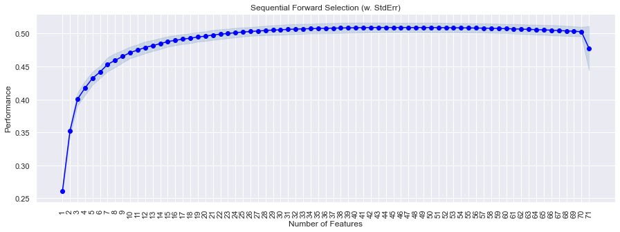
Selected Features: [2, 3]In real world scenario, you will review the performance changes with addition of each feature and choose a number of features that have considerable impact:
# to plot the performance with addition of each feature
from mlxtend.plotting import plot_sequential_feature_selection as plot_sfs

fig1 = plot_sfs(sfs.get_metric_dict(), kind="std_err", figsize=(15, 5))
plt.title("Sequential Forward Selection (w. StdErr)")
plt.xticks(rotation=90)
plt.show()

In example above, we can see that performance increases till the 30th feature and then slowly becomes constant, and then drops sharply after the 70th feature is added. The decision to choose the k_features now depend on the adjusted R2 vs the complexity of the model.
- With 30 features, we are getting an adjusted R2 of 0.506
- With 48 features, we are getting an adjusted R2 of 0.509.
- With 71 features, we are getting an adjusted R2 of 0.477.
The increase in adjusted R2 is not very significant as we are getting the same values with a less complex model. So we may use 30 features only to build our model.
